MVLib - Short Writeup - Version 5.0 Statistic, Signal filters, Fourier components - Last update: March 20, 2014 Source code available for local users only
In the second column of the following table, S stays for "Subroutine", I stays for "Integer function" and R stays for "Real function".
average(x,n)	R	Returns the average of the first n components of vector v.
sigma2(x,n)	R	Returns the variance of the first n components of vector v.
bias(x,y,n)	R	Returns the bias of the first n components of vectors x and y .
rmst(x,y,n)	R	Returns the Root Mean Square of the first n components of vectors x and y .
rmstn(x,y,n)	R	Returns the Normalized Root Mean Square of the first n components of vectors x and y .
vcorr(x,y,n)	R	Returns the absolute value of linear correlation coefficient of the first n components of vectors x and y, the coeffient ranges from 1 for a perfect correlation (or anticorrelation) to 0 for no correlation and is calculated as the absolute value of the following expression: .
wcorr(x,y,n)	R	Returns the linear correlation coefficient of the first n components of vectors x and y, the coeffient ranges from 1 for a perfect correlation to -1 for a perfect anticorrelation and is calculated as: .
rainscore(x,y,n,s,out)	S	Returns different statistic parameters for the first n components of two precipitation time series x and y, the real input argument s specifies the threshold and the results are returned in the components of vector out. out(1) will return the threat score ranging from 0 (very bad precipitation prediction) to 1 (perfect precipitation prediction); out(2) will return the FAI (False Alarm Index) ranging from 0 (perfect precipitation prediction) to 1 (very bad precipitation prediction): out(3) will return the normalized bias, if this value is the prediction is pefect, values greater/lower than this value shows an overestimation/underestimation.
nashsutcliffe(qo,qm,n)	R	Returns the Nash-Sutcliffe model efficiency coefficient. This coefficient is used to assess the predictive power of hydrological models. It is defined as: 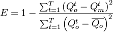where Qo is observed discharge, and Qm is modeled discharge. Qot is observed discharge at time t. Nash-Sutcliffe efficiencies can range from -inf to 1. An efficiency of 1 (E = 1) corresponds to a perfect match of modeled discharge to the observed data. An efficiency of 0 indicates that the model predictions are as accurate as the mean of the observed data, whereas an efficiency less than zero occurs when the observed mean is a better predictor than the model or, in other words, when the residual variance (described by the numerator in the expression above), is larger than the data variance (described by the denominator). See also: Nash, J. E. and J. V. Sutcliffe (1970), River flow forecasting through conceptual models part I - A discussion of principles, Journal of Hydrology, 10 (3), 282-290.
cioppskill(qo,qm,n)	R	Old version of nashsutcliffe routine documented above. This entry point is saved for backward compatibility only.
ttest(d1,n1,d2,n2)	R	Returns the T-test (or student test) to check the significancy of differences between two distributions, calculated as: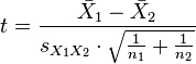 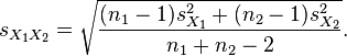where This test is used only when it can be assumed that the two distributions have the same variance. More details are available at Wikipedia page.
ttestthresh(n,sigma)	R	Returns the threshold value to be considered to evaluate the T-test (see routine ttest above), the first argument is the number of degree of freedom of distribution, the second real argument is the significancy level and the allowed values are: 0.9995, 0.999, 0.9975, 0.995, 0.99, 0.975, 0.95 and 0.90. Data are taken from the table reported at Wikipedia page.
Functions
sigmoide(x,a,b)	R	Returns the value of the sigmoid in the abscissa specified by the first argument; the second argument specifies the center of the sigmoid, the third argument specifies the distance from the center at which the sigmoid value is 0.1/0.9, namely the sigmoid is 0.1 when x=a-b and the sigmoid is 0.9 when x=a+b.
Random extraction
acaso(xx)	R	Returns a random number with a flat distribution in the range (0-1). The algorithm is platform independent and can be initialized using the MVLib parameter Random Seed. xx is a dummy argument.
gauss(average,sigma)	R	Returns a random number with a gaussian distribution. average is the average value and sigma is the standard deviation. The algorithm is platform independent and can be initialized using the MVLib parameter Random Seed.
Fourier Tranform
mvft(d,nd,a,b,n)	S	Calculates the first n coefficients of Fourier series for the first nd components of cevctor d, following: . The results are returned in the vectors a(0:n-1) and b(0:n-1). By definition is b(0)=0.
mvftinv(d,nd,a,b,n)	S	mvftinv carryout the inverse Fourier tranform. The first nd components of cevctor d are rebuilt using the n coefficients of Fourier series stored in the vectors a(0:n-1) and b(0:n-1).
mvftfilt(in,ou,n,ispett1,ispett2)	S	mvftfilt is medium frequencies filter. It rebuild in the vector out the n components of vector in, considering only the Fourier component between ispett1 and ispett2.
mvfthffilter(inp,out,n,a,b,c,w)	S	Allows to selecty the high frequencies in the n components of input real vector inp, the results are returned in the real vector out. The real vectors a and b will contain, as output, the smoothed Fourier coefficients. These coefficients are smoothed following a sigmoid function whose characteristic are specified by the real arguments c and w: the first specify the center of the sigmoid, the latter specify the width of the function, namely the value for which the sigmoid si smoothed by a factor 0.1/0.9; as an example if the arguments are n=200, c=100.0 and w=30.0, the component number 100 (the center of the sigmoide range) will be smoothed by a factor 0.5, the component number 130 will be smoothed by a factor 0.9 and the component number 70 will be smoothed by a factor 0.1. The sigmoid is calculated as follow:
mvfthffilter(inp,out,n,a,b,c,w)	S	Same as mvfthffilter but in this case low frequencies are selected, the sigmoid is this.
Signal filters
naverage (x,y,m,n)	S	The input vector x of m components is filtered with a n-average approach. The output vector y is calculated as
o1derivative(x,y,n)	S	The input vector x of n components is filtered with a first order derivative. The output vector y is calculated as
medianfilter(x,y,n,m)	S	The input vector x of n components is filtered with a median value calulated over m components. The result is returned in the real vector y.
dewmidnightfilter(y,ndata,noval,title)	S	Allows to filter the so called midnight bug of dewetra precipitation data. In many circumstances, the midnight data corresponds to the accumulated rain in the last N hours and N is often (but not always) 24. When the midnight value is anomalous respect the to values in the last 23 hours, the midnight value is set to no-data. The first argument is the time series, the second integer argument is the number of data (usually 8760 or 8784), the third integer argument is the no-data value (usually -9999), the last argument is a string, if this argument is not empty a log is produced by this routine.
d1cellcycle(vec,rule,dummy,n)	S	See the Cellular Automata routines description
cavectorfill(v,w,z,ndat)	S	See the Cellular Automata routines description
Quantic Normalization The following three subroutines allows to define and use a normalization to obtain a flat distribution from any observed distribution of data, this is carried out defining the value of tranformed distribution as: This is usually referred to as quantic normalization.
qnormdef(id,v,n)	S	The input vector x of n components is used to define the parameters of quantic normalization. The integer input flag id is not yet used, it can be used in the next versions to manipulate several normalization within the same application.
qnormal(id,x)	R	Returns the normalized value of input real argument x. The integer input flag id is not yet used.
qanormal(id,x)	R	Returns the annormalized value of input real argument x. The integer input flag id is not yet used.
Time series analisys
autocorrelation(x,n,y,lags)	S	Calculates the autocorrelation between the components of real vector x(n) considering an interval of 1-lags elements. The first component of output vector y will return the linear correlation between the elements x(i) and elements x(i+1); the k-th component of output vector y will return the linear correlation between the elements x(i) and elements x(i+k).
autocorrplot(x,n,y,lags)	S	Same as autocorrelation routine, but an histogram is also produced.