|
MVLib - Short Writeup - Version 4.0 Manipulating 1D and 2D arrays using Cellular Automata approach Last update: August, 20 2013 Source code available for local users only | |
| The following routines allow to manipulate 1-dimensional and 2-dimensional arrays characterized by continuous values. | |
| d2cellcycle(matr,rule,work,ix,jx,alpha) |
This routine carry out a cycle of evolution on the input real matrix
matr(ix,jx) passed as first argument, the input integer array
rule(ix,jx)contains the rules of evolution, while
real array work(ix,jx) is a work array, the last argument is
real coefficient specifyng the intensity of evolution the each cycle.
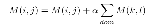
At each cycle each element of input array is modifield according to:
|
| d1cellcycle(vec,rule,dummy,n) |
The routine d1cellcycle is similar to previous one, but it works
on a one-dimensional array vec(n).
In this case the rules are specified in the integer vector passed as
second argument with the following meaning:
The third argument is a dummy argument for backward compatibility only and is NOT used by the routine. |
| cavectorfill(v,w,z,ndat) | This routine allows to fill the input real vector v(n) replacing the values -9999.0, usually marking a no-data value, with a value obtained as the average of the surrounding components of the vector (if you a sequence of more than 1 no-data values). The real vectors w(n) and z(n) are working arrays. It is used, as an example, to fill the observed time series before to plot them, see also the example 5. |
| The following routines allow to manipulate 2-dimensional arrays characterized by discrete values. | |
| cellularrule (conf,rule) |
cellularrule allows to define the evolution rules for a discrete
2-dimensional cellular automata system, to this aim you have to specify
the rules of evolution for each possible configuration. The first integer
argument specifies the configuration and the second integer argument
specifies the rule associated to this configuration. The cofiguration
are coded
taking into account the status of each bit, and the bits are numbered
clockwise from north-west (1) to west (8), as an example the configuration
where only the third bit is on
 is "called" 4, because it corresponds to the
bit configuration 00000100, if you want to specify the evolution rule
for this configuration you have to call cellularrule
specifying 4 as first argument. The second argument is coded value
specifying the rule of evolution, more specifically: is "called" 4, because it corresponds to the
bit configuration 00000100, if you want to specify the evolution rule
for this configuration you have to call cellularrule
specifying 4 as first argument. The second argument is coded value
specifying the rule of evolution, more specifically:
NB: The special value -1 for the first argument automatically allows to assign the rules of "Life game", in this case the second argument is ignored. See also the examples 38 and 40. The special value -2 for the first argument automatically allows to assign the rules for digital signal filtering, in this case the second argument is ignored. See also the example 39. |
| cellularinit(mat,m,n,type,xc,yc) | This routine allows to fill the array mat(m,n) with few standard macrostructures allowing to produce funny dynamical effects with Langton "Game of Life" rules; the kind of structure is specified by the integer parameter type passed as 4th argument (it must be in the range 1-3), the structure is created around the element of the matrix specified by the last two integer arguments. See also the examples 38 and 40. |
| cellularcycle(mat,m,n) | After defining the rules of evolution using cellularrule, this routine is invoked one or several times to preform a "life cycle" modify the integer input array mat(m,n). |
| cellularplot(mat,m,n) | This routine allows the plot the cellular automata system contained in the integer input array mat(m,n) passed as argument. See also the examples 38, 39 and 40. |
| cellularplotrule(flag,str) | Depending on the integer flag passed as argument, this routine allows to plot the naming of the rules (flag=0) or the rules defined at the current step (flag=1). The second argument is a string that will be used as prefix for the filename that will be created. See also the example 34. |
| MVLib documentation version 4.0 created by Marco Verdecchia | This document has been updated on February 27, 2013 h: 11.11 |